Types of Neural Networks

We can split neural networks into 2 categories based on their graph representation:

no cycles in the graph - vanilla network (ex: convolutional networks, classic deep networks) - stateless functions
cycles in the graph - recurrent neural networks (ex: text generation, continuous data anallysis) have internal memory - stateful (turing complete) programs

Feed-forward neural network

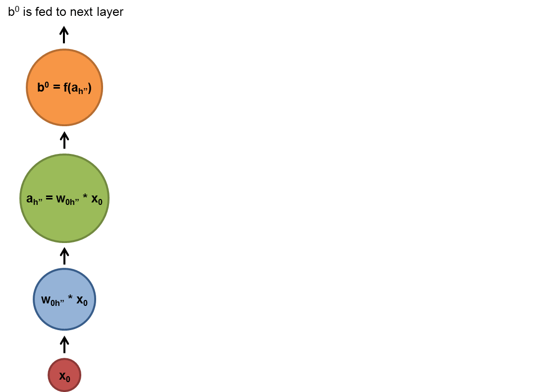
Most common type. It has an input layer, an output layer and a number of hidden layers (if > 1 then it is a ‘deep’ network). They compute a series of transformations that show the similarities between cases. The activities of neurons are a nonlinear function of the activities of the neurons in the previous layer.

Recurrent neural network

A RNN used shared parameters across time (instead of space as with a CNN), and they are useful for learning from and predicting sequences.

There are 2 types:

one to many: one input multiple outputs - we feed an input into the neural network, it gives an output, which we then feed back into the network; repeat this N times (ex: automatic image captioning)
many to one: many inputs one output - we give the network a sequence of inputs and at the end it will have one output (ex: text sentiment analysis)
many to many: many inputs - many outputs - we give the network a sequence of inputs and it will give back a sequence of outputs (ex: text translation)
synchronous many to many: many inputs - many outputs ; for each input we also use the information from the previous state of the network to produce a result (ex: video frame classification)

Have directed cycles in the connection graph. You may end up in the place you started. They are difficult to train and have complicated dynamics. They are more biologically realistic.

They can be used to model sequences, and develop a memory (they ‘remember’ information in the hidden states. It is very hard to train them to do so.

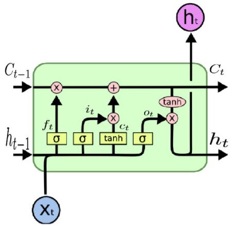
Memory cell

Since RNNs suffer from the vanishing gradient problem, that is backpropagating through time leads quickly to the derivatives becoming 0. Memory cells solve this problem by storing the value of the current output of the network.

LSTM - long short term memory

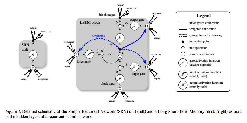
A LSTM memory cell with continuous input, output and forget functions

We have 4 building blocks:

- : element wise addition
x : element wise multiplication (used as gating, to allow a signal to be controlled by the output of the sigmoid function)
σ : sigmoid function applied to input
tanh : hyperbolic function applied to input

A memory cell has 3 basic operations:

write
read
forget

Compact form of the equations for the forward pass of an LSTM unit with a forget gate.12

\[\\begin{align} f_t &= \\sigma_g(W_{f} x_t + U_{f} h_{t-1} + b_f) \\\\ i_t &= \\sigma_g(W_{i} x_t + U_{i} h_{t-1} + b_i) \\\\ o_t &= \\sigma_g(W_{o} x_t + U_{o} h_{t-1} + b_o) \\\\ c_t &= f_t \\circ c_{t-1} + i_t \\circ \\sigma_c(W_{c} x_t + U_{c} h_{t-1} + b_c) \\\\ h_t &= o_t \\circ f_t(c_t) \\end{align}\]

f**t above is in our case tanh

W are weights used to modify x**t

U is the hidden state to state matrix, known as a transition matrix and similar to a Markov chain

b are biases

Variables and functions

x**t: input vector
h**t: hidden layer vector
y**t: output vector
W, U and b: parameter matrices and vector
σh* and *σy: activation functions

It’s important to note that LSTMs’ memory cells give different roles to addition and multiplication in the transformation of input. The central plus sign in both diagrams is essentially the secret of LSTMs. Stupidly simple as it may seem, this basic change helps them preserve a constant error when it must be backpropagated at depth. Instead of determining the subsequent cell state by multiplying its current state with new input, they add the two, and that quite literally makes the difference. (The forget gate still relies on multiplication, of course.)3

GRU - gated recurrent unit

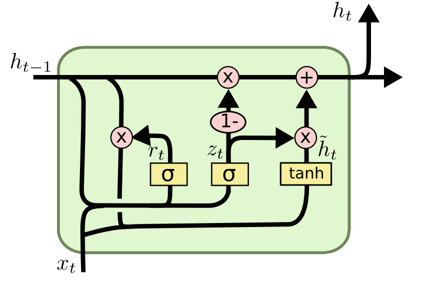
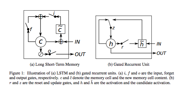
Initially, for t = 0, the output vector is h0 = 0.

\[\\begin{align} z_t &= \\sigma_g(W_{z} x_t + U_{z} h_{t-1} + b_z) \\\\ r_t &= \\sigma_g(W_{r} x_t + U_{r} h_{t-1} + b_r) \\\\ h_t &= (1-z_t) \\circ h_{t-1} + z_t \\circ \\sigma_h(W_{h} x_t + U_{h} (r_t \\circ h_{t-1}) + b_h) \\end{align}\]

The last function applies EWMA to filter the output of the current layer based on the output of the last layers.

Because this feedback loop occurs at every time step in the series, each hidden state contains traces not only of the previous hidden state, but also of all those that preceded h_t-1 for as long as memory can persist.

Rolling window

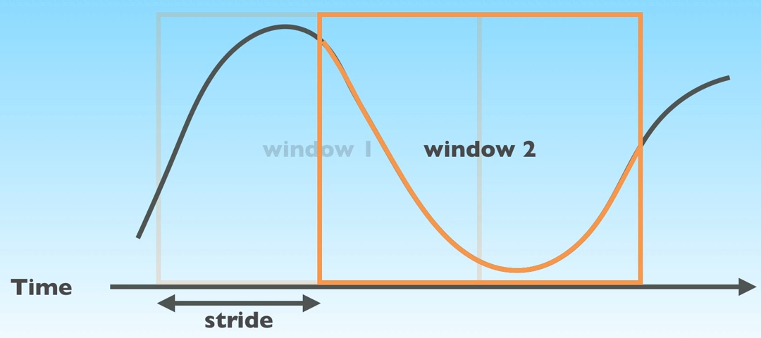
To optimally train a RNN we can use the rolling window approach. Instead of predicting the output based on one data point, we predict the output based on a sequence of inputs.

Beam search

Let’s say we are trying to predict a sequence of words. We can try to predict N words at a time, and keep the most probable combination. But this is time consuming since each step of the prediction is exponentially larger than the last. For this we can use beam search, at each step of our prediction we prune the combinations that have a low likelihood.

Applications

Ilya Sutskever trained one of these networks to predict the next character in a sequence (using data from Wikipedia). Generated text: “In 1974 Northern Denver had been overshadowed by CNL, and several Irish intelligence agencies in the Mediterranean region. However, on the Victoria, Kings Hebrew stated that Charles decided to escape during an alliance. The mansion house was completed in 1882, the second in its bridge are omitted, while closing is the proton reticulum composed below it aims, such that it is the blurring of appearing on any well-paid type of box printer.”

Since they can predict sequences from singular inputs or other sequences, they can be used in many ways. For example you can put the output of a CNN as the input and have the RNN try to generate captions. Or use them to translate sequences of text from one language to another.

But you need lots of training data and compute time.

Advice

Here are a few ideas to keep in mind when manually optimizing hyperparameters for RNNs:

Watch out for overfitting, which happens when a neural network essentially “memorizes” the training data. Overfitting means you get great performance on training data, but the network’s model is useless for out-of-sample prediction.
Regularization helps: regularization methods include l1, l2, and dropout among others.
So have a separate test set on which the network doesn’t train.
The larger the network, the more powerful, but it’s also easier to overfit. Don’t want to try to learn a million parameters from 10,000 examples – parameters > examples = trouble.
More data is almost always better, because it helps fight overfitting.
Train over multiple epochs (complete passes through the dataset).
Evaluate test set performance at each epoch to know when to stop (early stopping).
The learning rate is the single most important hyperparameter. Tune this using deeplearning4j-ui; see this graph
In general, stacking layers can help.
For LSTMs, use the softsign (not softmax) activation function over tanh (it’s faster and less prone to saturation (~0 gradients)).
Updaters: RMSProp, AdaGrad or momentum (Nesterovs) are usually good choices. AdaGrad also decays the learning rate, which can help sometimes.
Finally, remember data normalization, MSE loss function + identity activation function for regression, Xavier weight initialization

Symmetrically connected neural networks

Like recurrent networks, but have the same weight in both directions(the connections are symmetric). They are easier to analyze than recurrent networks, but are more restricted in what they can do (they obey an energy function). If they have no hidden layers they are called Hopfield nets.

Symmetrically connected neural networks with hidden layers

They are called Boltzmann machines. More powerful than Hopfield nets, less powerful than recurrent networks. Beautifully simple learning algorithm.

Convolutional Neural Networks

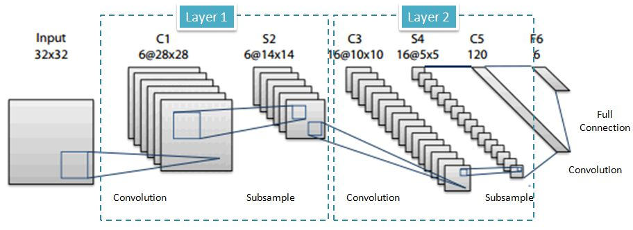
In machine learning, a convolutional neural network (CNN, or ConvNet) is a class of deep, feed-forward artificial neural networks, most commonly applied to analyzing visual imagery.

CNNs use a variation of multilayer perceptrons designed to require minimal preprocessing. They are also known as shift invariant or space invariant artificial neural networks (SIANN), based on their shared-weights architecture and translation invariance characteristics.4

In each layer of the network we take a convolution (let’s say a 5x5 convolution), and we run it across the image. Each layer of the image is known as a featuremap. By doing this we generate new feature maps. Next, we subsample those featuremaps and repeat the process. At the final layer we will have a large number of 1x1 feature maps that we feed into our neural network.

Parameters:

Kernel size - for ex 5x5
Input depth - for ex RGB = 3
Output depth
Padding - what do you do at the edge of the image?
- Valid - don’t go beyond the edge of the image
- Same - pad the image with 0s
Stride - the number of pixels by which you shift your kernel each turn

For example your images input Tensor will have the shape: (N, H, W, C):

N - number of images
H - height of images
W - width of images
C - number of channels in each image

Your kernels Tensor will have the shape: (Hf, Wf, Ci, Co):

Height of filter patch
Width of filter patch
Number of input channels
Number of output channels

Subsampling

Subsampling can be acomplished using pooling, which can either be:

mean pooling - each pixel in the subsampled feature map takes the value of the average of those in the polling section
max pooling - each pixel in the subsamples feature map takes the value of the maximum of those in the polling section

For pooling we can adjust:

polling method
polling size (the size of the square which gets compressed into 1 pixel into the new feature map)

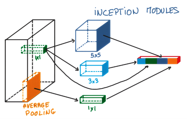
1x1 convolutions

We can add a 1x1 convolution between our feature maps and our kernels. It’s a cheap an inexpensive way to enhance our network.

Inception module

input_img = Input(shape = (32, 32, 3))

tower_1 = Conv2D(64, (1,1), padding='same', activation='relu')(input_img)
tower_1 = Conv2D(64, (3,3), padding='same', activation='relu')(tower_1)

tower_2 = Conv2D(64, (1,1), padding='same', activation='relu')(input_img)
tower_2 = Conv2D(64, (5,5), padding='same', activation='relu')(tower_2)

tower_3 = MaxPooling2D((3,3), strides=(1,1), padding='same')(input_img)
tower_3 = Conv2D(64, (1,1), padding='same', activation='relu')(tower_3)

output = keras.layers.concatenate([tower_1, tower_2, tower_3], axis = 3)

Since there are so many choices for valid kernels and polling parameters, why choose? The inception model combines multiple kernels/pollings into one feature map.