Linear algebra is the branch of mathematics concerning linear equations.
Based on this course: Essence of linear algebra by 3Blue1Brown
Vectors
Vectors are nx1 dimensional matrices. They can be added together element wise, or multiplied with scalars (numbers). Graphically then can be represented as arrows from the origin of the coordinate system to the point defining them.
Think of single vectors as line segments, think of multiple vectors as points.
When adding 2 vectors, we move the second one so that it’s tail is at the top of the first one, then draw a line connecting the origin with the top of the second vector.
Linear combination of vectors
$a\vec{v}+b\vec{w}$
If you keep a or b constant and vary the value of the other one, you will get a straight line.
The set of vectors you can reach using any linear combination of n vectors is called the span of those vectors.
If one of the vectors can be removed without reducing the span, we say the n vectors are linearly dependent(one of the vectors can be expressed as a linear combination of the others). If on the other hand each vector adds a new dimension to the span they are said to be linearly independent
For 2D there are 3 posibilities:
- vectors are linearly dependent, and their span is a line
- vectors are linearly independent and their span is the whole 2D plane
- vectors are 0, their span is the point (0,0)
Basis
A basis of a space is a set of linearly independent vectors whose span is that space.
For the 2d coordinate system we use $\hat{i}$ and $\hat{j}$ as a basis.
Changing bases
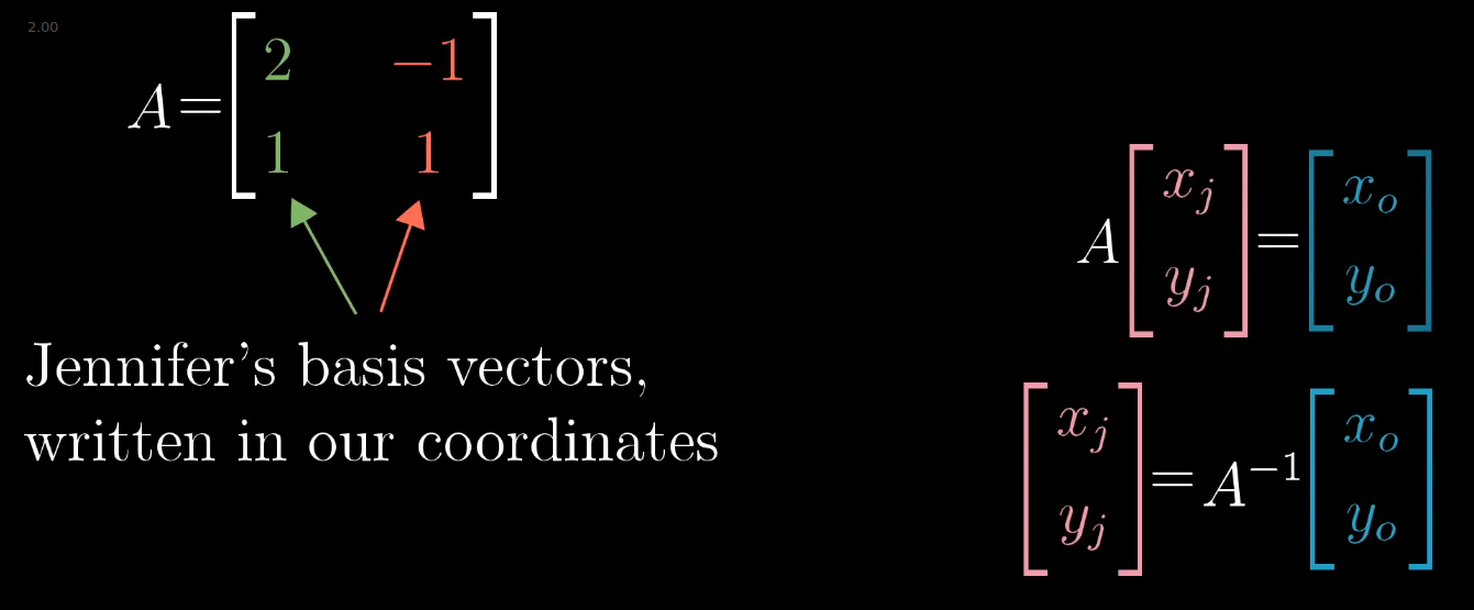
If we want to represent a vector with a different basis, we can use a linear transformation. That linear transformation would be a matrix with the new basis vectors as columns.
To translate one of our vectors into a different basis we multiply our vector by the inverse of that basis’ transformation matrix.
To apply a transformation in a different basis.
$A^{-1} * M * A * \vec{v}$Apply transformation M described in basis B1 to vector v described in B2 with the base transformation matrix B2->B1 A.
Eigenvectors
An eigen vector is a vector that remains on its span after a transformation. Its eigenvalue is the factor by which it gets stretched/squished.
In 3D space, if we have a rotation transformation, finding its eigenvector = finding the axis of rotation.
$A*\vec{v} = \lambda*\vec{v}$ where A is a transformation, v an eigenvector and lambda its eigenvalue
To solve: $A*\vec{v} = (\lambda*I)*\vec{v} (A - \lambda*I)*\vec{v} = \vec{0} A - \lambda*I = \vec{0}$
Eigenbasis
If all the vectors that form our basis are eigen vectors, it means our basis is an eigenbasis, represented by a diagonal matrix.
This is nice because multiplying diagonal matrices is easy. So if we want to repeatedly apply a transformation, we can try to change its input to an eigenbasis, compute it there than change the result back to our basis.
Linear transformations / operations
Formal definition:
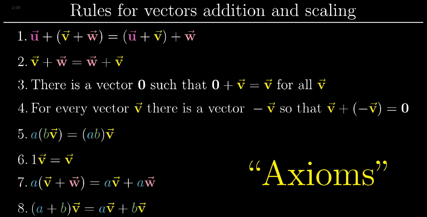
An operation L is linear if it has the following 2 properties:
- Additivity: $L(\vec{v}+\vec{w}) = L(\vec{v})+L(\vec{w})$
- Scaling: $L(c\vec{v})=cL(\vec{v})$
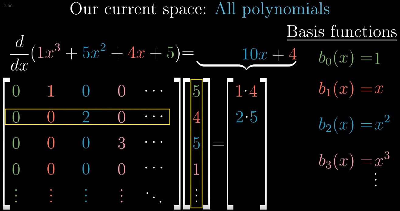
We call it a transformation if it is applied to vectors, operation if it is applied to functions (ex: derivative).
All lines must remain lines (no curbing). The origin has to be fixed. Imagine transformation as being applied to the whole plane.
For example: if we take the vector $\vec{a} = 1*\hat{i}-2*\hat{j}$, after a linear transformation $transform(\vec{a}) = 1*transform(\hat{i})-2*transform(\hat{j})$
Any 2D linear transformation can be quantified by 4 numbers:
- 2 representing where $\hat{i}$ lands
- 2 representing where $\hat{j}$ lands
$\begin{bmatrix} i_x & j_x \
i_y & j_y \end{bmatrix}$
Applying the transformation to a vector:
$\begin{bmatrix} a & b \
c & d \end{bmatrix} * \begin{bmatrix} x \
y \end{bmatrix} = x*\begin{bmatrix} a \
c \end{bmatrix} +y* \begin{bmatrix} b \
d \end{bmatrix} = \begin{bmatrix} a*x + b*y \
c*x + d*y \end{bmatrix}$
Matrix multiplications as compositions
If we have 2 matrices that we want to apply successively to transform a given vector, we can apply their composition to the vector to achieve the same result in one step.
Example: let’s say we have a rotation and a shear we want to apply to a vector. We can calculate their composition and apply it to the vector.
$\begin{bmatrix} 1 & 1 \
0 & 1 \end{bmatrix} * \begin{bmatrix} 0 & -1 \
1 & 0 \end{bmatrix} = \begin{bmatrix} 1 & -1 \
1 & 0 \end{bmatrix}$
shear * rotation = composition
Note: we apply the transformations from right to left. The same way we compose functions g(f(x)).
Space orientation
At first $\hat{i}$ is to the right of $\hat{j}$. If after a transformation $\hat{i}$ is to the left $\hat{j}$, it means that the orientation of space has been inverted.
Column space
The column space of a matrix A is the set of all the possible outputs of $A\vec{v}$. It’s also called the span of the columns.
Rank
The rank of a transformation is the number of dimensions at its output. If it squishes space into a line then it’s rank is 1, if it squishes space into a plane than it’s rank is 2. For a 2x2 matrix the max rank is 2.
More precise definition: rank = number of dimensions in the column space.
Null space/Kernel
The null space or kernel of your matrix is the set of all vectors that, after the transformation land in the origin. (for a 2D matrix with rank 1, a whole line of vectors lands in the origin; for a 3D matrix with rank 1 a whole plane of vectors lands in the origin).
In the case of equations($A*\vec{x}=\vec{v}$, if $\vec{v}$ is null, null space gives you all of the solutions for your equation.
Determinants
A determinant is a measure of how a transformation changes the area of the square determined by $\hat{i}$ and $\hat{j}$. In 3D space it tells us how much volumes are changing.
If the determinant is 0, the transformation squishes everything into a smaller dimension.
If the determinant is negative, it means the orientation of space has been inverted. For 3D space we can use the 3 finger rule: forefinger for i, thumb for k and middle finger for j. If you can do this after the transformation it means orientation has not changed.
Inverse
A−1 is the transformation that, when applied after A gives the identity transformation I, that has ones on the main diagonal and zeroes everywhere else. A−1 * A = I
The inverse only exists if det(A) > 0
Non Square Matrices
Non square matrices map inputs to outputs of different dimensions. For example a 3x2 matrix maps 2D vectors into 3D space.
Dot product
A ⋅ B = sum(A.*B)
We can remember this easily in the following form: $\hat{i}*\hat{j}=+1$
Between 2 vectors:
- If they point in the same direction $\vec{v}\cdot \vec{w}>0$
- If they are perpendicular $\vec{v}\cdot \vec{w}=0$
- If they point in opposite directions $\vec{v}\cdot \vec{w}<0$
Cross product
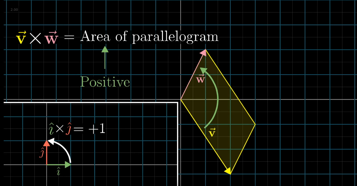
2D space
The cross product $\vec{v}\times \vec{w}$ is equal to the area defined by the parallelogram with the sides resting on v and w. We have 3 cases:
- v is to the right of w, v x w > 0
- v = w, v x w = 0
- v is to the left of w, v x w < 0
3D space
In the 3D space, the cross product is a vector of length = area of parallelogram and perpendicular to it (direction given by 3 finger rule)
$\begin{bmatrix} v1 \
v2 \
v3 \end{bmatrix} \times \begin{bmatrix} w1 \
w2 \
w3 \end{bmatrix} = \det{( \begin{bmatrix} \hat{i} & v1 & w1 \
\hat{j} & v2 & w2 \
\hat{k} & v3 & w3 \end{bmatrix} )}$
Duality
Every time we have a transformation that takes us to the number line, we can think of it as a vector; and applying the transformation is identical to doing a dot product with that vector.
Matrices
Orthogonal matrices
In linear algebra, an orthogonal matrix is a square matrix whose columns and rows are orthogonal unit vectors (i.e., orthonormal vectors), i.e.
QTQ = QQT = I, where I is the identity matrix.
This leads to the equivalent characterization: a matrix Q is orthogonal if its transpose is equal to its inverse:
Q**T = Q−1.
An orthogonal matrix Q is necessarily:
- Invertible (with inverse: 1 = Q−1 = Q**T
- Unitary 1 = Q−1 = Q*
- Normal 1 = Q* * Q = Q * Q* in the reals.
The determinant of any orthogonal matrix is either +1 or −1. As a linear transformation, an orthogonal matrix preserves the dot product of vectors, and therefore acts as an isometry of Euclidean space, such as a rotation or reflection. In other words, it is a unitary transformation.
Markov chains
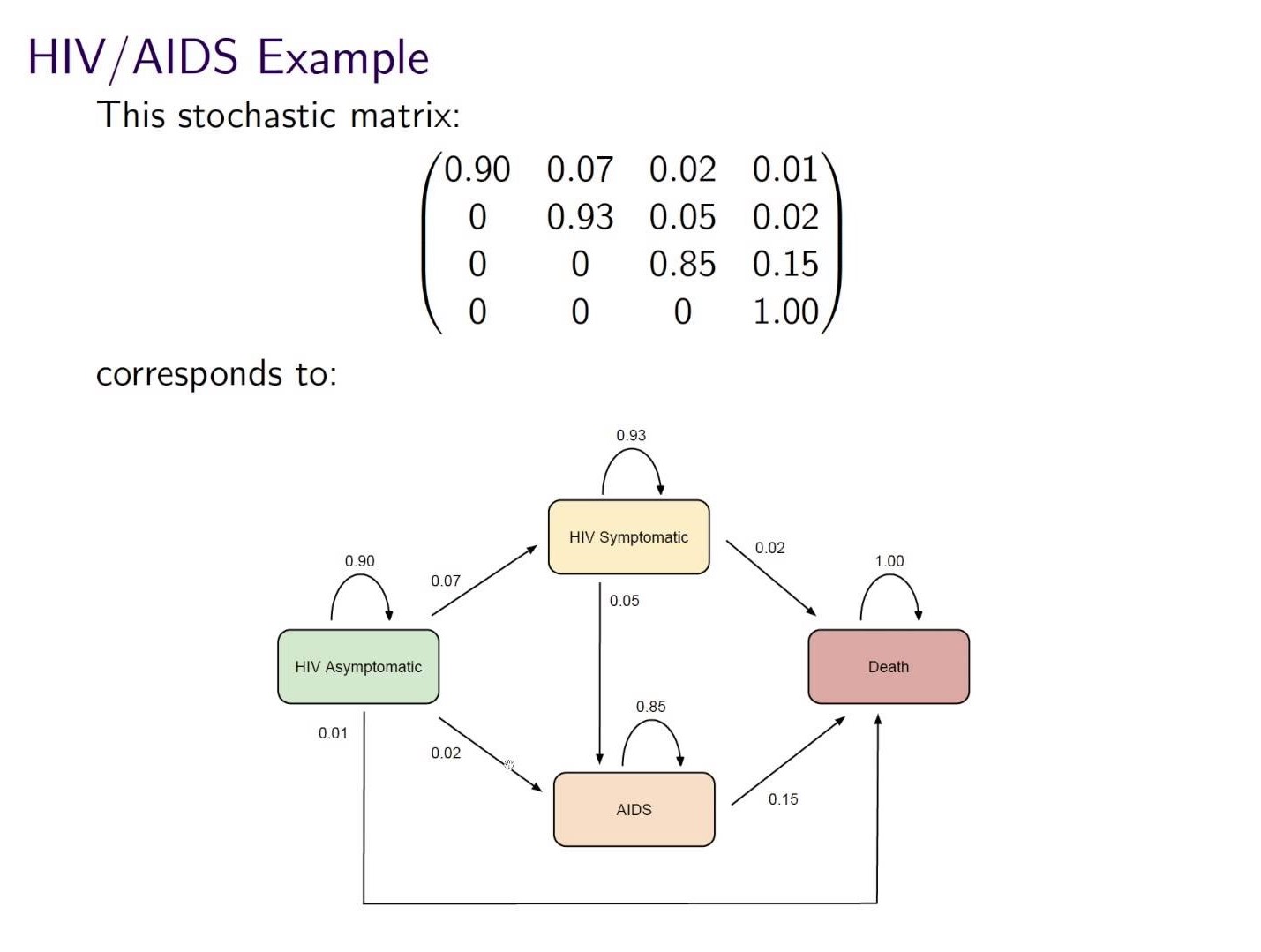
Markov chains are expressed as stochastic matrices, with each entry Mij representing the probability of jumping from state i to state j. The row sum of such a matrix is always 1.