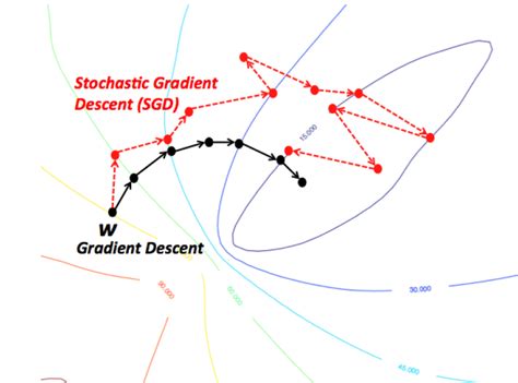
(Batch) Gradient Descent
m = number of training examples
n = number of features
Cost: $J_{train}(\theta)=\frac{1}{2m}\sum_{i=1}^mh_\theta(x^{(i)}-y^{(i)})^2$
Repeat{ $\theta_j := \theta_j - \alpha \frac{1}{m}\sum_{i=1}^mh_\theta(x^{(i)}-y^{(i)})x_j^{(i)}$(j=0:n) }for
Stochastic Gradient Descent
$cost(\theta,(x^{(i)},y^{(i)})) = \frac{1}{2}h_\theta(x^{(i)}-y^{(i)})^2$
Cost \(J_{train}(\\theta)=\\frac{1}{m}\\sum_{i=1}^mcost(\\theta,(x^{(i)},y^{(i)}))\)
Repeat{ for i=1:m{ θj* := *θj − αhθ(x(i) − y(i))x**j(i)(j=0:n) } }for - usually 1-10
Convergence
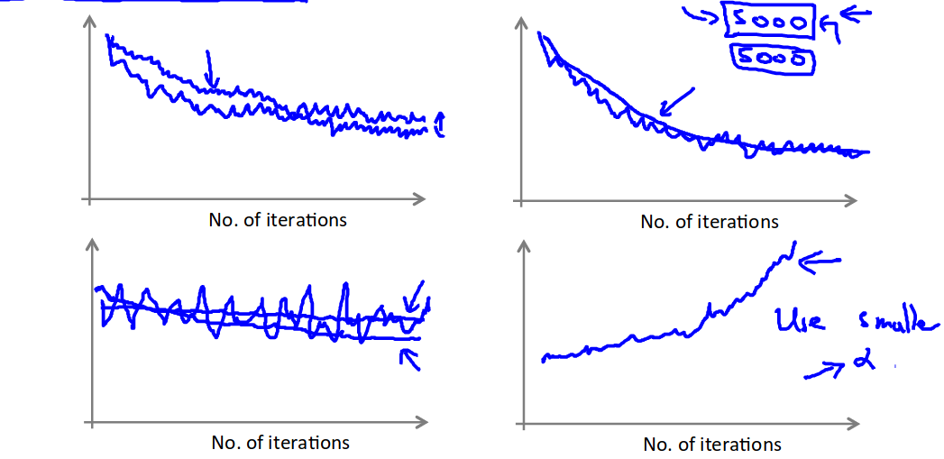
Compute ost(θ, (x(i), y(i))) before each update to θ. Every plot the cost average over the last iterations
Mini batch gradient descent
Imagine b(number of examples in batch)=10, m=1000
Repeat{ for i=1,11,21,...991{ $\theta_j := \theta_j - \alpha \frac{1}{m}\sum_{k=i}^{i+9}h_\theta(x^{(i)}-y^{(i)})x_j^{(i)}$(j=0:n) } }for
Online learning
For instance searches on a website, or purchases on a website.
Repeat{ Get(x,y) Update θ θj* := *θj − αhθ(x − y)x**j(j=0:n) }forever
Powerful as it can adapt to user preference changes in time.
Map Reduce and Parallelism
We map the test test set into a number of chunks depending on how many machines/cpu cores we want to use, then we process each chunk in parallel, then add up the result on one of the machines/cpu cores.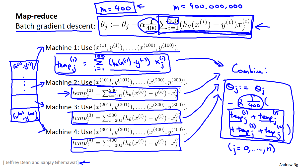 <figcaption>border</figcaption>