Deep learning is a new way to teach machines by giving them lots of data, and having them process it in ways only humans could before. Compared to other machine learning techniques, deep learning systems profit more from complex models, huge amounts of data and a longer computation time.
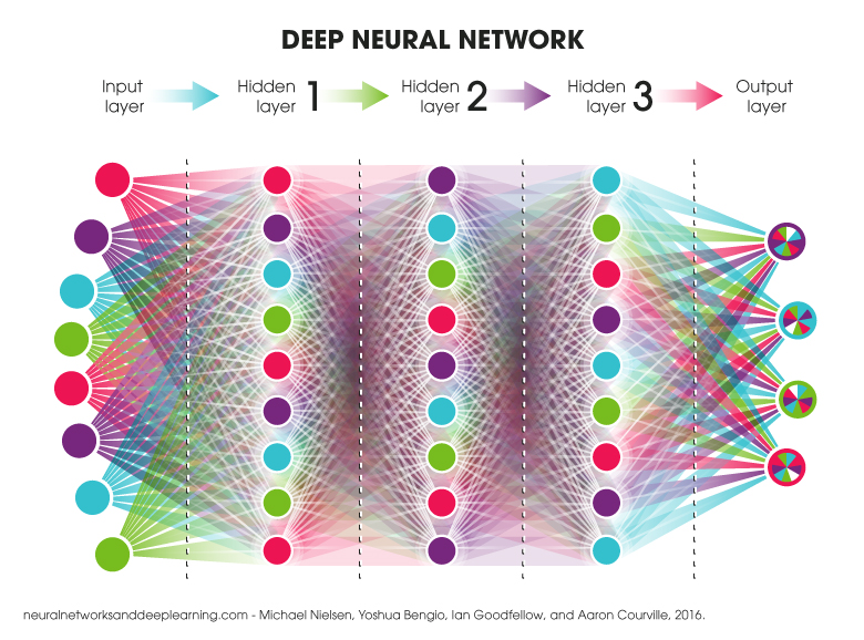
When I say deep learning I think of a multi-layered neural network.
Basics
Simple network
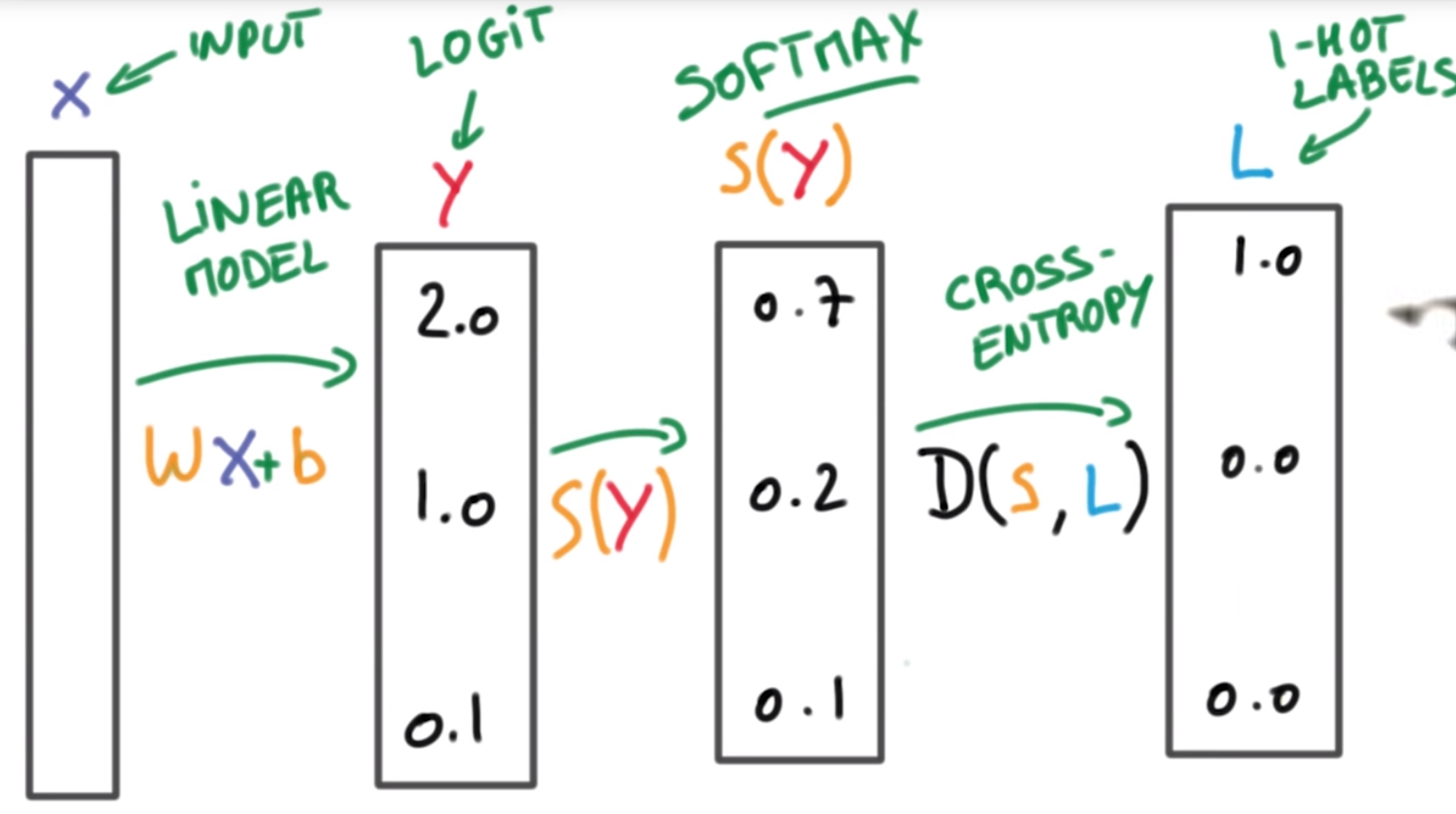
To train our NN we will set an optimization objective. In this case it will be minimizing our cost function J.
$J(\theta)=\frac{1}{m}\sum_{i=1}^mD(h_\theta(\theta_i*x_i+b),L_i)$where D is the cross entropy function, and L is a matrix of hot encoded labels
Data preprocessing
Standard normalization
We want our data to have μ(mean)=0 and σ(Xi)=σ(Xj) for any j!=i (variance).
from sklearn.preprocessing import StandardScaler

ss = StandardScaler()
df['data_ss'] = ss.fit_transform(df[[/'data'|'data']])
df.describe().round(2)
MinMax normalization
We’ll scale our data to fit on a scale from 0.0 to 1.0
from sklearn.preprocessing import MinMaxScaler

mms = MinMaxScaler()
df['data_mms'] = mms.fit_transform(df[[/'data'|'data']])
df.describe().round(2)
Weight initialization
We’ll initialize our weights from a Gaussian distribution with μ=0 and standard deviation σ. If we pick a small σ, the algorithm will be more uncertain (your output predictions will be relatively equal at first), if we pick a large σ you algorithm will be more opinionated (your output predictions will have spikes).
One hot encoding
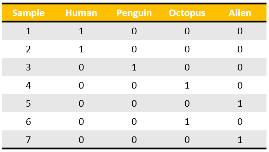
One hot encoding transforms categorical features to a format that works better with classification and regression algorithms.1
Imagine we have 7 samples belonging to 4 categories, OHE will output a 4x1 vector (represented below as a row of the table) for each of them.
Hyperparameter optimization2
In our neural networks we have a number of hyperparameters we can tune (learning rate, batch size, optimizer type etc.). In order to tune this we usually have a master that controls many workers performing experiments (training the network with a certain combination of parameters for a number of epochs) and returning results.
Steps:
- decide on a value for the hyperparameters
We have a couple of ways to search for good hyperparameter combinations:
- random search
- grid search
- Bayesian optimization
Random search
Randomly chooses values for the parameters. Can outperform grid search when a small number of hyper parameters affects the final performance of the network.
Grid search
Exhaustive searching through a manually defined parameter space, usually guided by a metric calculated on the cross validation set. Continuous parameters will need to be turned into discrete sets of values.
Bayesian search
Bayesian optimization build a probabilistic model function that maps from the hyperparameter space to the objective on the cross validation set, which gets updated after each new observation. The aim is to find the minimum of that function. In practice is has been shown to be better than random / grid search.
Gradient based optimization
Try to compute the gradient with respect to the hyperparameters and use it to optimize them.
Evolutionary optimization
Evolutionary optimization is a methodology for the global optimization of noisy black-box functions. In hyperparameter optimization, evolutionary optimization uses evolutionary algorithms to search the space of hyperparameters for a given algorithm.3 Evolutionary hyperparameter optimization follows a process inspired by the biological concept of evolution:
- Create an initial population of random solutions (i.e., randomly generate tuples of hyperparameters, typically 100+)
- Evaluate the hyperparameters tuples and acquire their fitness function (e.g., 10-fold cross-validation accuracy of the machine learning algorithm with those hyperparameters)
- Rank the hyperparameter tuples by their relative fitness
- Replace the worst-performing hyperparameter tuples with new hyperparameter tuples generated through crossover and mutation
- Repeat steps 2-4 until satisfactory algorithm performance is reached or algorithm performance is no longer improving
Evolutionary optimization has been used in hyperparameter optimization for statistical machine learning algorithms4, automated machine learning56, deep neural network architecture search78, as well as training of the weights in deep neural networks9.
Activation functions
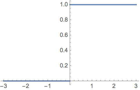
Step
step(x) = x > 0
Sigmoid
$sigmoid(x) = \frac{1}{1-\exp{(-x)}}$
Hyperbolic Tangent(tanh)
output(x) = tanh(x)
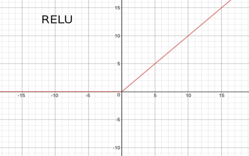
ReLU(rectified linear unit)
relu(x) = max(0,x)
Softplus
softplus(x) = log(1 + exp(x))

Softmax
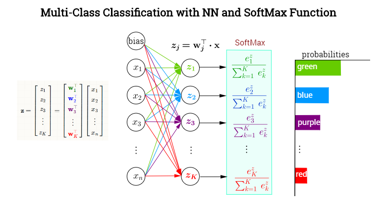
In mathematics, the softmax function, or normalized exponential function, is a generalization of the logistic function that “squashes” a K-dimensional vector z of arbitrary real values to a K-dimensional vector σ(z) of real values, where each entry is in the range (0, 1), and all the entries add up to 1.10
They are used after last layer of a neural network to turn a vector of values into a vector of probabilities in the range[0,1] with the total sum of the vector being 1.
$\sigma(z)j=\frac{e^{z_j}}{\sum{k=1}^Ke^{z_k}}$
Optimization11
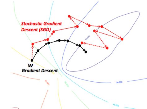
(Batch) Gradient Descent
m = number of training examples
n = number of features
Cost: $J_{train}(\theta)=\frac{1}{2m}\sum_{i=1}^mh_\theta(x^{(i)}-y^{(i)})^2$
Repeat{ $\theta_j := \theta_j - \alpha \frac{1}{m}\sum_{i=1}^mh_\theta(x^{(i)}-y^{(i)})x_j^{(i)}$(j=0:n) }for
Stochastic Gradient Descent
$cost(\theta,(x^{(i)},y^{(i)})) = \frac{1}{2}h_\theta(x^{(i)}-y^{(i)})^2$
Cost \(J_{train}(\\theta)=\\frac{1}{m}\\sum_{i=1}^mcost(\\theta,(x^{(i)},y^{(i)}))\)
Repeat{ for i=1:m{ θj* := *θj − αhθ(x(i) − y(i))x**j(i)(j=0:n) } }for - usually 1-10
Convergence
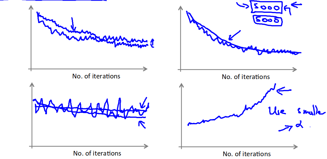
Compute ost(θ, (x(i), y(i))) before each update to θ. Every plot the cost average over the last iterations
Mini batch gradient descent
Imagine b(number of examples in batch)=10, m=1000
Repeat{ for i=1,11,21,...991{ $\theta_j := \theta_j - \alpha \frac{1}{m}\sum_{k=i}^{i+9}h_\theta(x^{(i)}-y^{(i)})x_j^{(i)}$(j=0:n) } }for
Online learning
For instance searches on a website, or purchases on a website.
Repeat{ Get(x,y) Update θ θj* := *θj − αhθ(x − y)x**j(j=0:n) }forever
Powerful as it can adapt to user preference changes in time.
Map Reduce and Parallelism
We map the test test set into a number of chunks depending on how many machines/cpu cores we want to use, then we process each chunk in parallel, then add up the result on one of the machines/cpu cores.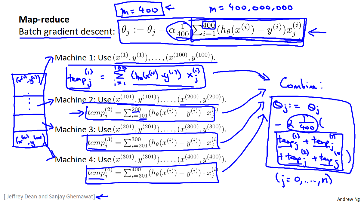 <figcaption>border</figcaption>
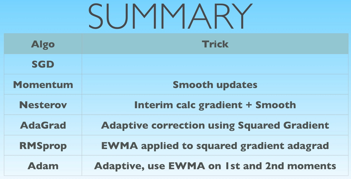
SGD with momentum
v is a k dimensional vector of the same dimensions as θ; it will be our gradient step
v0 = ∇θ0 * L(θ0, X, y);θ − weight* *matrix, ∇θ − gradien**t w.r.t.θ Calculate gradient at step 0
vt* = *β* * *vt − 1 + (1 − β)*∇θt* − 1 * *L*(*θt − 1, X, y);β − momentu**mCalculate gradient at step t; we use a Weighed Moving Average
θt* = *θt − α * v**tTake a step
Momentum defines how much of the step is determined by the previous gradient step, and how much by the current gradient. Usually momentum = 0.9
AdaGrad12
Authors present AdaGrad in the context of projected gradient method – they offer non-standard projection onto parameters space with the goal to optimize certain entity related to regret. Final AdaGrad update rule is given by the following formula:
Gk* = *Gk − 1 + ∇J(θ**k − 1)2
$\theta^k = \theta^{k-1} - \frac{\alpha}{\sqrt{G^{k-1}}}*\nabla*J(\theta^{k-1})$
where * and sqrt are element wise
G is the historical gradient information. For each parameter we store sum of squares of its all historical gradients – this sum is later used to scale/adapt a learning rate. In contrast to SGD, AdaGrad learning rate is different for each of the parameters. It is greater for parameters where the historical gradients were small (so the sum is small) and the rate is small whenever historical gradients were relatively big.
“Informally, our procedures give frequently occurring features very low learning rates and infrequent features high learning rates, where the intuition is that each time an infrequent feature is seen, the learner should “take notice.” Thus, the adaptation facilitates finding and identifying very predictive but comparatively rare features” – original paper
In any case though learning rate descreases from iteration to iteration – to reach zero at infinity. That is btw considered a problem and solved by authors of AdaDelta algorithm.
AdaDelta13
Adadelta mixes two ideas though – first one is to scale learning rate based on historical gradient while taking into account only recent time window – not the whole history, like AdaGrad. And the second one is to use component that serves an acceleration term, that accumulates historical updates (similar to momentum).
Adadelta update rule consists of the following steps:
- Compute gradient g**t at current time t
- Accumulate gradients: E[g2]t = ρ * E[g2]t − 1 + (1 − ρ)*g**t2 layout: wiki_post base: Wiki base_url: /wiki categories:
- wikimisc
- Accumulate updates(momentum like): E[Δx*2]*t* = *ρE[Δx*2]*t* − 1 + (1 − *ρ*)*Δx**t2 layout: wiki_post base: Wiki base_url: /wiki categories:
- wikimisc
ρ is a decay constant (a parameter) and ϵ is there for numerical stability (usually very small number).
We choose epsilon to be 10−6 – in original AdaDelta paper though epsilon is considered to be a parameter. We don’t go there now to limit hyper-parameter space (but in fact different results are reported for different values of epsilon in original paper)
RMSProp14
vt* = ∇*θt − 1 * L(θ**t − 1, X, y)Calculate gradient step
$E_t = \beta * E_{t-1} + (1-\beta)*v_t^2 ; \beta - momentum:\ number\ of\ steps\ remembered\ \frac{1}{1-\beta}(\beta=0.9 => 10\ steps), E - exponentially\ weighed\ moving\ average\ of\ the\ gradient\ squared$If my gradient is consistently small it will be a big number; if my gradient is volatile or consistently large it will be a big number
$\theta_t = \theta_{t-1} - \alpha * \frac{v_t}{\sqrt{E_t}}$Take the step
This means that if our gradient is consistently small we’ll take bigger jumps, and if it is volatile or too big we’ll take smaller jumps
Adam15
vt* = *β*1 * *vt − 1 + (1 − β1)*∇θt* − 1 * *L*(*θt − 1, X, y),β1 − first order momentu**mCalculate gradient step with momentum
Et* = *β*2 * *Et − 1 + (1 − β2)*vt*2; *β* − *second order momentum*, *E* − *exponentially* *weighed* *moving average of* *the* *gradient squaredIf my gradient is consistently small it will be a big number; if my gradient is volatile or consistently large it will be a big number
$\theta_t = \theta_{t-1} - \alpha * \frac{v_t}{\sqrt{E_t}}$Take the step
This means that if our gradient is consistently small we’ll take bigger jumps, and if it is volatile or too big we’ll take smaller jumps + we’ll jump in the previous direction (RMSProp with momentum basically)
Choosing the best optimizer
According to Optimization techniques comparison in Julia: SGD, Momentum, Adagrad, Adadelta, Adam
All of the algorithms perform differently depending on the problem and parametrization. AdaGrad is the best with the shallow problem (softmax classifier), AdaDelta is somewhere between all others – never leads, never fails badly too. Momentum and classical SGD seem to be a good fit to any problem of the above – they both produce leading results often. Adam has his big moment minimizing error of network #3 (with a bit worse accuracy there).
For all of the methods the most challenging part is how to choose proper parameters values. And there is no clear rule for that too, unfortunately. The one ‘solid’ conclusion that can be drawn here is “to choose whatever works best for your problem” – I’m afraid. Although starting with simple methods – classical SGD or momentum – might be enough very often following what the experiments show.
Implementation-wise optimization techniques presented here do not differ between one another that much too, some of the algorithms expect a bit more computations and storage, but they all share the same linear complexity with respect to number of parameters – choosing simpler methods might win another vote then.
Regularization
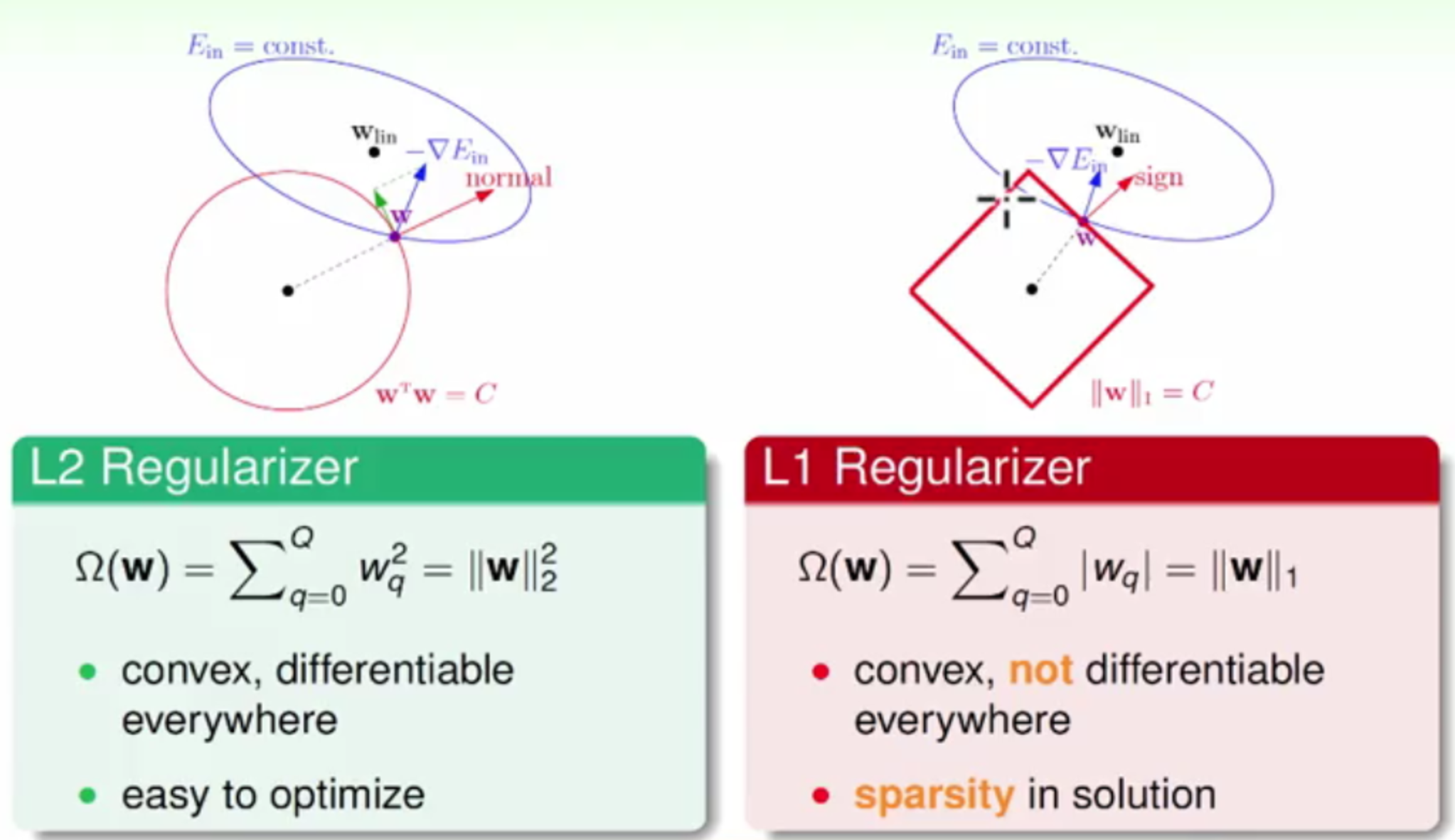
We have 2 ways to regularize our network, L1 and L2. What these do is add another term to the cost function, which penalizes the network proportional to the values of the weights.
Batch Normalization 16
Input: values of x(activation of a layer) over a minibatch B = {x1…m}
Parameters to be learned: γ, β
$\mu_B = \frac{1}{m} \sum_{i=1}^{m}x_i$ mini batch mean
$\sigma_B^2 = \frac{1}{m} \sum_{i=1}^{m}(x_i - \mu_B)^2$ mini batch variance
$\hat{x_i} = \frac{x_i - \mu_B}{\sqrt{\sigma_B^2 + \epsilon}}$ normalization
Finally
$y_i = \gamma * \hat{x_i} + \beta \equiv BN_{\gamma, \beta}(x_i)$ scale and shift
Important notes:
The last step of batch normalization is the most important.
We usually use a EWMA of μB* *and* *σB2 calculated across previous minibatches, with a momentum of 0.1
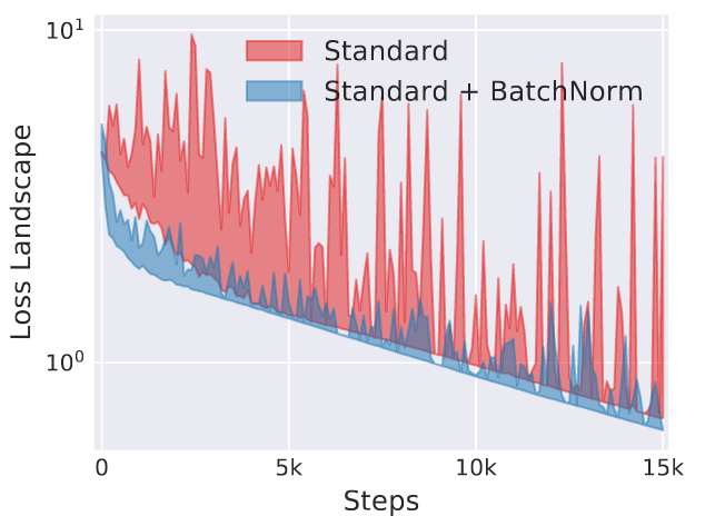
Why it helps? 17
It reduces the bumpiness of the loss landscape, allowing us to use higher learning rates.
Example:
Imagine we’re predicting movie reviews, and we have ratin**g = f(θ, X); rating should be in the range [0,5], but f may produce values in the range [-1,1]; the scale and mean are of
Let’s modify f: rating* = *f*(*θ*, *X*)**γ* + *β* *γ*, *β* − *learnable* *parameters; γ provides a direct gradient for scale, and β provides a direct gradient for mean
Now it is easy for f to give an output in the range [0,5]
Local Response Normalization18
With this answer I would like to summarize contributions of other authors and provide a single place explanation of the LRN (or contrastive normalization) technique for those, who just want to get aware of what it is and how it works.
Motivation: ‘This sort of response normalization (LRN) implements a form of lateral inhibition inspired by the type found in real neurons, creating competition for big activities among neuron outputs computed using different kernels.’ AlexNet 3.3.
In other words LRN allows to diminish responses that are uniformly large for the neighborhood and make large activation more pronounced within a neighborhood i.e. create higher contrast in activation map. prateekvjoshi.com states that it is particulary useful with unbounded activation functions as RELU.
Original Formula: For every particular position (x, y) and kernel i that corresponds to a single ‘pixel’ output we apply a ‘filter’, that incorporates information about outputs of other n kernels applied to the same position. This regularization is applied before activation function. This regularization, indeed, relies on the order of kernels which is, to my best knowledge, just an unfortunate coincidence.
In practice (see Caffe) 2 approaches can be used:
- WITHIN_CHANNEL. Normalize over local neighborhood of a single channel (corresponding to a single convolutional filter). In other words, divide response of a single channel of a single pixel according to output values of the same neuron for pixels nearby.
- ACROSS_CHANNELS. For a single pixel normalize values of every channel according to values of all channels for the same pixel
Actual usage LRN was used more often during the days of early convets like LeNet-5. Current implementation of GoogLeNet (Inception) in Caffe often uses LRN in connection with pooling techniques, but it seems to be done for the sake of just having it. Neither original Inception/GoogLeNet (here) nor any of the following versions mention LRN in any way. Also, TensorFlow implementation of Inception (provided and updated by the team of original authors) networks does not use LRN despite it being available.
Conclusion: Applying LRN along with pooling layer would not hurt the performance of the network as long as hyper-parameter values are reasonable. Despite that, I am not aware of any recent justification for applying LRN/contrast normalization in a neural-network.
Keras implementation19
class LRN(Layer):
    def __init__(self, alpha=0.0001,k=1,beta=0.75,n=5, **kwargs):
      self.alpha = alpha
      self.k = k
      self.beta = beta
      self.n = n
      super(LRN, self).__init__(**kwargs)

    def call(self, x, mask=None):
      b, ch, r, c = x.shape
      half_n = self.n // 2 # half the local region
      input_sqr = T.sqr(x) # square the input
      extra_channels = T.alloc(0., b, ch + 2*half_n, r, c) # make an empty tensor with zero pads along channel dimension
      input_sqr = T.set_subtensor(extra_channels[:, half_n:half_n+ch, :, :],input_sqr) # set the center to be the squared input
      scale = self.k # offset for the scale
      norm_alpha = self.alpha / self.n # normalized alpha
      for i in range(self.n):
          scale += norm_alpha * input_sqr[:, i:i+ch, :, :]
      scale = scale ** self.beta
      x = x / scale
      return x

    def get_config(self):
      config = {"alpha": self.alpha,
          "k": self.k,
          "beta": self.beta,
          "n": self.n}
      base_config = super(LRN, self).get_config()
      return dict(list(base_config.items()) + list(config.items()))
Embeddings20
How do we build a neural network for text processing? Words that appear very often, like ‘the’, don’t tell us very much, while rare words, like ‘retinopathy’ might tell us a lot about the text.
- We’d like to see important words often enough to understand their meaning
- We’d like to understand how words relate to each other
For this we’d need to collect A LOT of labeled data, so much in fact, that we’re going to turn to unsupervised learning.
The internet is full of texts that we can train on if we figure out what to learn from them. Powerful idea: similar words tend to occur in similar contexts.
We’re going to turn each of our words into a small vector called an embedding. Our model should group semantically similar words together using their embedded representation, such as the distance between the embeddings of similar words is small.
Skip-gram
Skip-gram idea: we will train our algorithm to take a word and predict it’s context given the word. For instance, given ‘one’ the algorithm might say ‘two’, or ‘five’.
- Get a text corpus; I used the one from here: [mattmahoney.net/dc/ Data Compression Programs]
- Decide how big your vocabulary is gonna be; let’s say 50,000 words, and put your first 50,000 most repeated words into a dictionary which will map a word to its index; all other words will be mapped into an entry labeled ‘UNK’
- Convert your text corpus into a list of indices in the dictionary you just built
- Create a function to generate batches of training data and labels from your dictionary
- It will be parametrized with: batch_size, num_skips and skip_window
- batch_size = how many examples to use for each optimizer pass
- num_skips = how many times to reuse an input to generate a label
- skip_window = how many nearby words to consider context
- Train a skip-gram model
- Calculate word contexts by the distance between the 2 words’ embeddings
Example data generated with batch_size 8: data: ['anarchism', 'originated', 'as', 'a', 'term', 'of', 'abuse', 'first'] with num_skips = 2 and skip_window = 1: batch: ['originated', 'originated', 'as', 'as', 'a', 'a', 'term', 'term'] labels: ['as', 'anarchism', 'a', 'originated', 'as', 'term', 'of', 'a'] with num_skips = 4 and skip_window = 2: batch: ['as', 'as', 'as', 'as', 'a', 'a', 'a', 'a'] labels: ['a', 'anarchism', 'term', 'originated', 'as', 'of', 'originated', 'term']
End
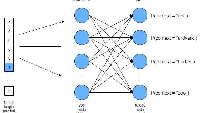
CBOW (Continuous bag of words)
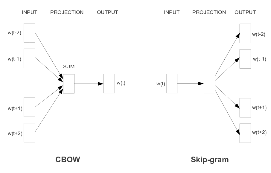
We’re going to train our model to take a context and predict a word from it. Imagine we give it the words: ‘anarchism’, ‘originated’, x, ‘a’, ‘term’; it should predict x = ‘as’
- Get a text corpus; I used the one from here: [mattmahoney.net/dc/ Data Compression Programs]
- Decide how big your vocabulary is gonna be; let’s say 50,000 words, and put your first 50,000 most repeated words into a dictionary which will map a word to its index; all other words will be mapped into an entry labeled ‘UNK’
- Convert your text corpus into a list of indices in the dictionary you just built
- Create a function to generate batches of training data and labels from your dictionary
- It will be parametrized with: batch_size and R
- batch_size = how many examples to use for each optimizer pass
- R = number of words to consider before the given word and after it; so, for R=2 we would take 2 words before the word and 2 words after it
- Train a CBOW model, which takes 2*R inputs, averages them, and then tries to predict a word
- Give it a context and see what word it outputs
Example data generated with batch_size 8: data: ['anarchism', 'originated', 'as', 'a', 'term', 'of', 'abuse', 'first', 'used', 'against', 'early', 'working', 'class', 'radicals', 'including', 'the'] with R= 1: batch 0 : ['anarchism', 'as'] batch 1 : ['originated', 'a'] batch 2 : ['as', 'term'] batch 3 : ['a', 'of'] batch 4 : ['term', 'abuse'] batch 5 : ['of', 'first'] batch 6 : ['abuse', 'used'] batch 7 : ['first', 'against'] labels: ['originated', 'as', 'a', 'term', 'of', 'abuse', 'first', 'used'] with R= 2: batch 0 : ['anarchism', 'originated', 'a', 'term'] batch 1 : ['originated', 'as', 'term', 'of'] batch 2 : ['as', 'a', 'of', 'abuse'] batch 3 : ['a', 'term', 'abuse', 'first'] batch 4 : ['term', 'of', 'first', 'used'] batch 5 : ['of', 'abuse', 'used', 'against'] batch 6 : ['abuse', 'first', 'against', 'early'] batch 7 : ['first', 'used', 'early', 'working'] labels: ['as', 'a', 'term', 'of', 'abuse', 'first', 'used', 'against']
Architectures
ResNet
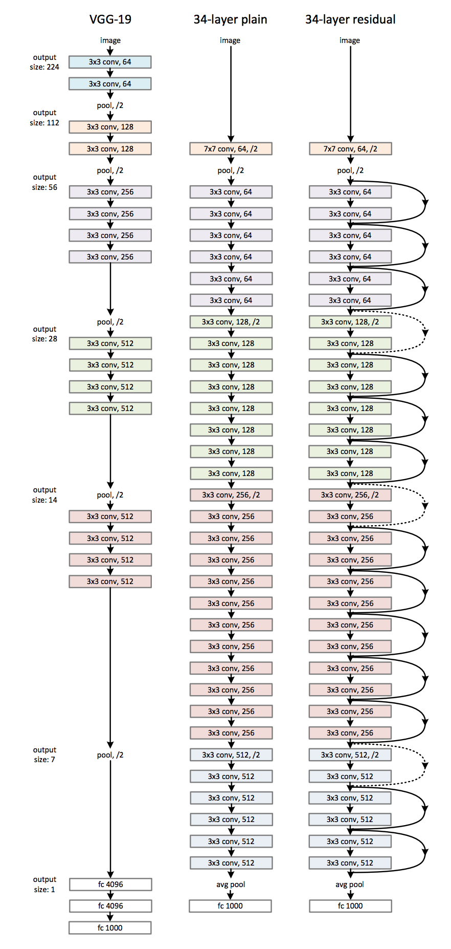
ResNets use feedforward identity connections
Wide ResNet 21
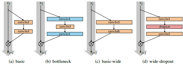
Wide ResNet uses wider blocks to make the networks easier to train to the same accuracy as the older ones.
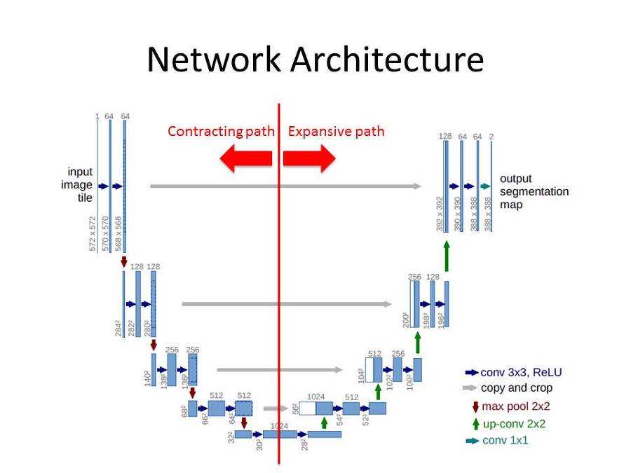
UNet
3
4
5
6
7
8
9