Reinforcement learning is an important type of Machine Learning where an agent learn how to behave in a environment by performing actions and seeing the results.
Inspired greatly by: An introduction to Reinforcement Learning by Thomas Simonini
The idea behind Reinforcement Learning is that an agent will learn from the environment by interacting with it and receiving rewards for performing actions.
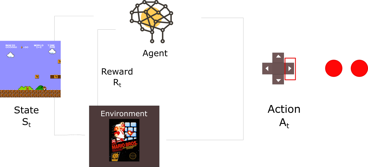
Let’s imagine an agent learning to play Super Mario Bros as a working example. The Reinforcement Learning (RL) process can be modeled as a loop that works like this:
- Our Agent receives state S0 from the Environment (In our case we receive the first frame of our game (state) from Super Mario Bros (environment))
- Based on that state S0, agent takes an action A0 (our agent will move right)
- Environment transitions to a new state S1 (new frame)
- Environment gives some reward R1 to the agent (not dead: +1)
This RL loop outputs a sequence of state, action and reward. The goal of the agent is to maximize the expected cumulative reward.
Reward
The cumulative reward at each time step t:
Gt* = *Rt + 1 + R**t + 2 + … equivalent to $G_{t}=\sum_{k=0}^{T} R_{t+k+1}$
Rewards are discounted in time (with a factor gamma) to account for the fact that future rewards now are better than rewards in the future.
$G_{t}=\sum_{k=0}^{\infty} \gamma^{k} R_{t+k+1} \text { where } \gamma \in[0,1)$
Task types
Episodic
In this case, we have a starting point and an ending point (a terminal state). This creates an episode: a list of States, Actions, Rewards, and New States.
For instance think about Super Mario Bros, an episode begin at the launch of a new Mario and ending: when you’re killed or you’re reach the end of the level.
Continous
These are tasks that continue forever (no terminal state). In this case, the agent has to learn how to choose the best actions and simultaneously interacts with the environment.
For instance, an agent that do automated stock trading. For this task, there is no starting point and terminal state. The agent keeps running until we decide to stop him.
Learning methods
Monte Carlo (learning once / episode)
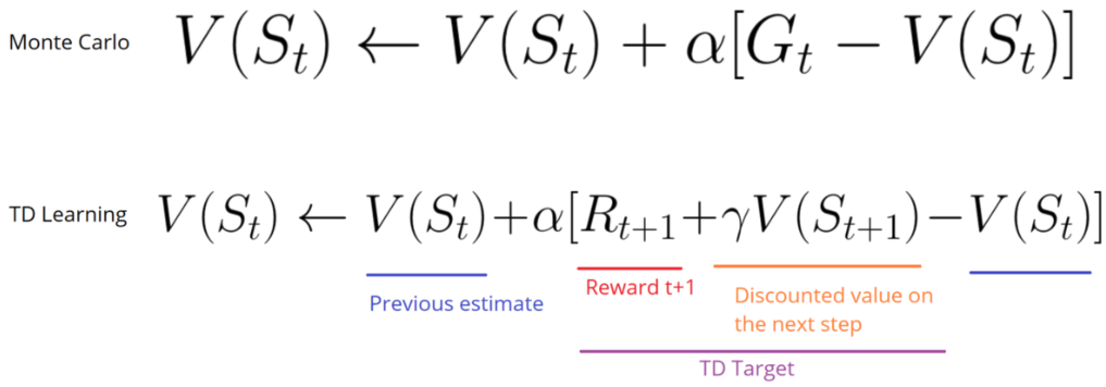
Monte Carlo When the episode ends (the agent reaches a “terminal state”), the agent looks at the total cumulative reward to see how well it did. In Monte Carlo approach, rewards are only received at the end of the game.
Then, we start a new game with the added knowledge. The agent makes better decisions with each iteration.
V(St*) ← *V*(*St) + α[Gt*−*V*(*St)]
V(St*) − *maximumexpectedfuturerewardstartingatthelaststat**e
Temporal Difference Learning (learning at each timestep)
V(St*) ← *V*(*St) + α[Rt* + 1+*γV(St* + 1)−*V*(*St)]
TD methods only wait until the next time step to update the value estimates. At time t+1 they immediately form a TD target using the observed reward Rt+1 and the current estimate V(St+1).
Exploration vs Exploitation
- Exploration is finding more information about the environment.
- Exploitation is exploiting known information to maximize the reward.
Epsilon greedy strategy
- We specify an exploration rate “epsilon,” which we set to 1 in the beginning. This is the rate of steps that we’ll do randomly. In the beginning, this rate must be at its highest value, because we don’t know anything about the values in Q-table. This means we need to do a lot of exploration, by randomly choosing our actions.
- We generate a random number. If this number > epsilon, then we will do “exploitation” (this means we use what we already know to select the best action at each step). Else, we’ll do exploration.
Three approaches to Reinforcement Learning
Value Based
In value-based RL, the goal is to optimize the value function V(s).
The value function is a function that tells us the maximum expected future reward the agent will get at each state.
The value of each state is the total amount of the reward an agent can expect to accumulate over the future, starting at that state.
| vπ*(*s*)=𝔼*π*[*Rt + 1+γRt + 2+γ2R**t + 3+… | S**t=s] |
The agent will use this value function to select which state to choose at each step. The agent takes the state with the biggest value.
Policy Based
In policy-based RL, we want to directly optimize the policy function π(s) without using a value function.
The policy is what defines the agent behavior at a given time.
a = π(s)
We learn a policy function. This lets us map each state to the best corresponding action.
We have two types of policy:
- Deterministic: a policy at a given state will always return the same action.
- Stochastic: output a distribution probability over actions.
Model Based
In model-based RL, we model the environment. This means we create a model of the behavior of the environment.
The problem is each environment will need a different model representation.
Value based Reinforcement Learning algorithms
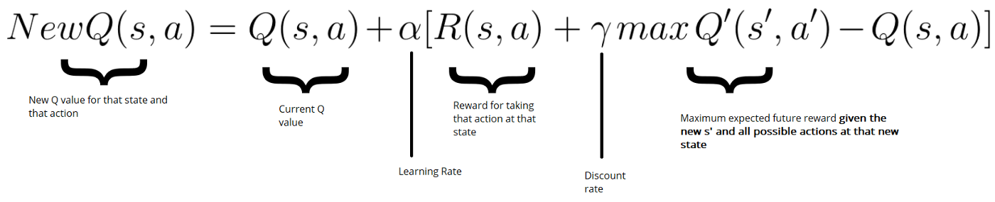
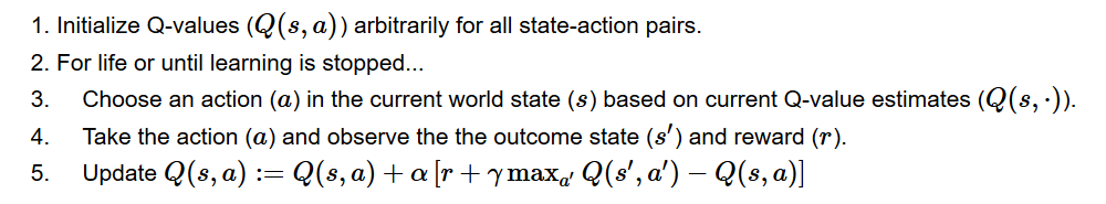
Q learning
We will create a table where we’ll calculate the maximum expected future reward, for each action at each state. In terms of computation, we can transform this grid into a table. This is called a Q-table (“Q” for “quality” of the action).
Learning the Action Value Function (Q - function)
| Qπ*(*st,at*) = *E*[*Rt + 1+γRt + 2+γ2R**t + 3+… | st*,*at] |
We can see this Q function as a reader that scrolls through the Q-table to find the line associated with our state, and the column associated with our action. It returns the Q value from the matching cell. This is the “expected future reward.”
Deep Q Learning
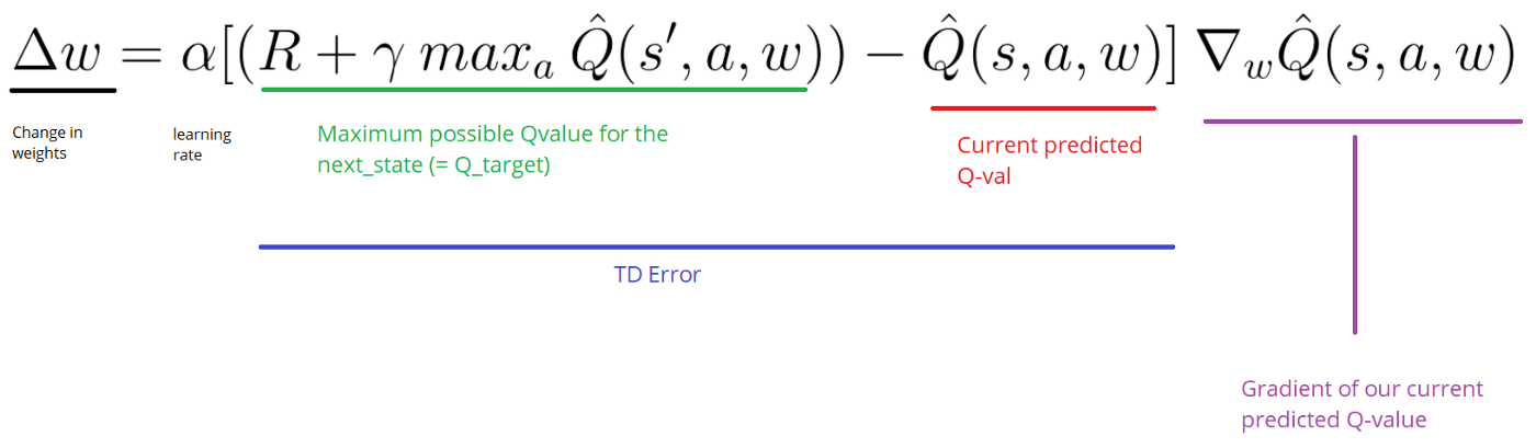
Instead of using a Q-table, we’ll implement a Neural Network that takes a state and approximates Q-values for each action based on that state.
The error (or TD error) is calculated by taking the difference between our Q_target (maximum possible value from the next state) and Q_value (our current prediction of the Q-value)
Whilst training, we can choose to retain a replay memory M, with some capacity N, from which we will train the algorithm. This helps the network’s “memory”, and prevents it from only learning about what it has immediately done.
Fixed Q targets
Using a separate network with a fixed parameter (let’s call it w-) for estimating the TD target. After T time steps w- <- w (we update the fixed parameters).
Double DQNs
When we compute the Q target, we use two networks to decouple the action selection from the target Q value generation. We:
- use our DQN network to select what is the best action to take for the next state (the action with the highest Q value).
- use our target network to calculate the target Q value of taking that action at the next state.
Dueling DQN
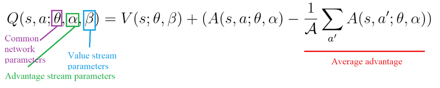
So we can decompose Q(s,a) as the sum of:
- V(s): the value of being at that state
- A(s,a): the advantage of taking that action at that state (how much better is to take this action versus all other possible actions at that state).
Q(s, a)=A(s, a)+V(s)
With DDQN, we want to separate the estimator of these two elements, using two new streams:
- one that estimates the state value V(s)
- one that estimates the advantage for each action A(s,a)
Prioritized experience replay 1
Prioritized Experience Replay (PER) was introduced in 2015 by Tom Schaul. The idea is that some experiences may be more important than others for our training, but might occur less frequently.
Because we sample the batch uniformly (selecting the experiences randomly) these rich experiences that occur rarely have practically no chance to be selected.
We want to take in priority experience where there is a big difference between our prediction and the TD target, since it means that we have a lot to learn about it.
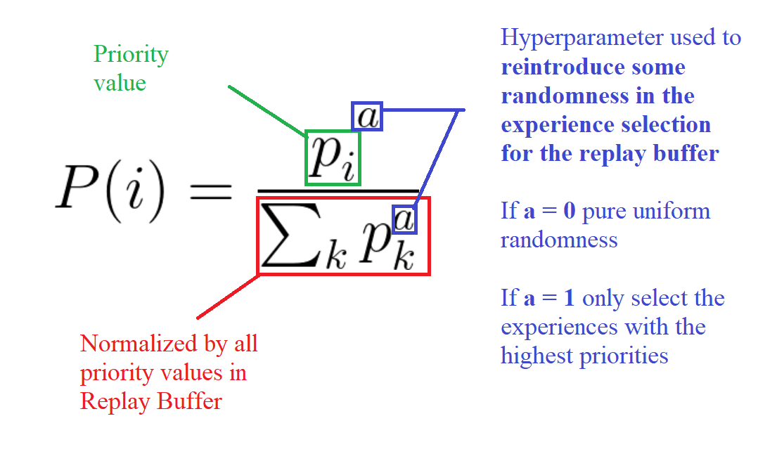
| We add to each entry in our replay buffer a probability p**t = | δ**t | + ϵ |
But we can’t just do greedy prioritization, because it will lead to always training the same experiences (that have big priority), and thus over-fitting.
So we introduce stochastic prioritization, which generates the probability of being chosen for a replay.
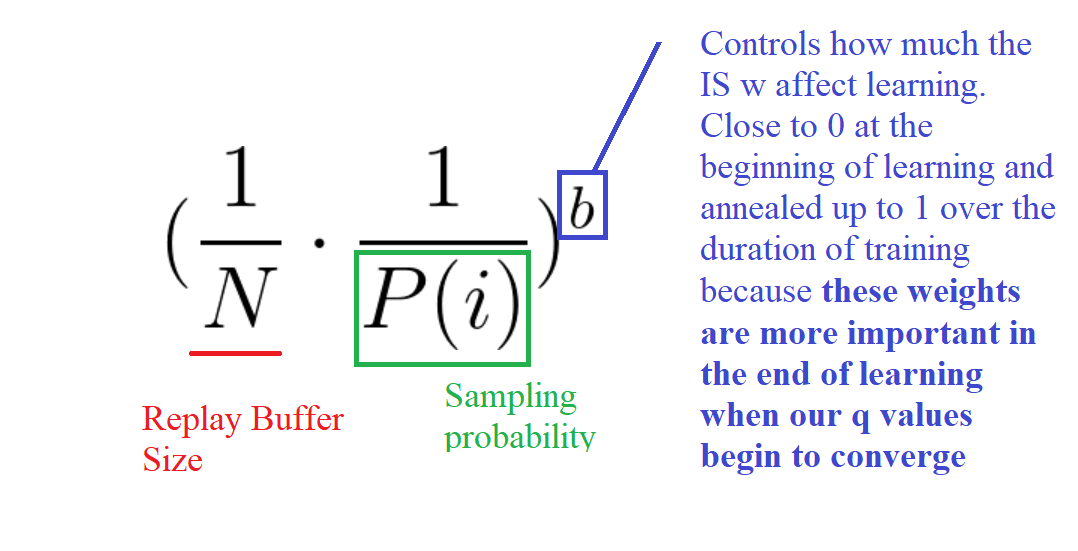
But, because we use priority sampling, purely random sampling is abandoned. As a consequence, we introduce bias toward high-priority samples (more chances to be selected).
To correct this bias, we use importance sampling weights (IS) that will adjust the updating by reducing the weights of the often seen samples.
Policy based Reinforcement Learning algorithms
There are 2 types of policies:
- deterministic: given state s, π(s)=a
stochastic: given state s, π(a s)=P(a**t s**t) (Partially Observable Markov Decision Process (POMDP))
Stochastic policies are the most common type.
Main advantages:
- convergence: because we follow the gradient to find the best parameters, we’re guaranteed to converge on a local maximum (worst case) or global maximum (best case)
- better in high dimensional action spaces: if we have a high number of continuous actions, policy based methods can model them better
- policy gradients can learn stochastic policies
Disadvantages:
- they tend to converge on a local optima
- longer training times
Objective/Policy Score function
J1(θ)=Eπ*[*G*1=*R*1+*γR2+γ2R3+…] = E**π(V(s1))
The idea is simple. If I always start in some state s1, what’s the total reward I’ll get from that start state until the end?
In a continuous environment, we can use the average value, because we can’t rely on a specific start state.
Each state value is now weighted (because some happen more than others) by the probability of the occurrence of the respected state.
$J_{avgv}(\theta)=E_{\pi}(V(s))=\sum d(s) V(s){\ where \ }d(s)=\frac{N(s)}{\sum_{s^{\prime}} N\left(s^{\prime}\right)}\ (the frequency of the state)$
Third, we can use the average reward per time step. The idea here is that we want to get the most reward per time step.
JavR*(*θ*)=*Eπ(r)=∑sd*(*s*)∑*aπθ*(*s*, *a*)*Rs**a (probability that I’m in state s) (probability that I take action a from that state under this policy) (immediate reward)
Gradient ascent
Our goal is to find the parameter θ that maximizes J(θ).
J(θ)=Eπ*[*R*(𝒯)], *where* 𝒯 = (*si, ai*, *ri) (expected given policy) (expected future reward)
Which is the total summation of expected reward given policy.
Hybrid method
Actor Critic (A2C)
We’ll using two neural networks:
- a Critic that measures how good the action taken is (value-based)
- an Actor that controls how our agent behaves (policy-based)
The Actor Critic model is a better score function than Monte Carlo. Instead of waiting until the end of the episode as we do in Monte Carlo REINFORCE, we make an update at each step (TD Learning).